import numpy as np
import matplotlib.pyplot as plt
%matplotlib inline
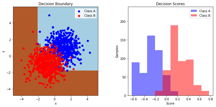
here we start with the most popular classification algorithm in high energy physics; the Boosted Descision Tree.
This is a ensemble classifier so needs two imports. We generate random gaussian blobs to classify.
from sklearn.ensemble import AdaBoostClassifier
from sklearn.tree import DecisionTreeClassifier
from sklearn.datasets import make_gaussian_quantiles
# Construct dataset
X1, y1 = make_gaussian_quantiles(mean=(1,1), cov=1,
                                 n_samples=500, n_features=2,
                                 n_classes=1, random_state=1)
X2, y2 = make_gaussian_quantiles(mean=(-1, -1), cov=1,
                                 n_samples=500, n_features=2,
                                 n_classes=1, random_state=1)
X = np.concatenate((X1, X2))

y = np.concatenate((y1, - y2 + 1))
X.shape
(1000, 2)
# Create and fit an AdaBoosted decision tree
bdt = AdaBoostClassifier(DecisionTreeClassifier(max_depth=1),
                         algorithm="SAMME",
                         n_estimators=200)
bdt.fit(X, y)
AdaBoostClassifier(algorithm='SAMME',
          base_estimator=DecisionTreeClassifier(class_weight=None, criterion='gini', max_depth=1,
            max_features=None, max_leaf_nodes=None,
            min_impurity_decrease=0.0, min_impurity_split=None,
            min_samples_leaf=1, min_samples_split=2,
            min_weight_fraction_leaf=0.0, presort=False, random_state=None,
            splitter='best'),
          learning_rate=1.0, n_estimators=200, random_state=None)
plot_colors = "br"
plot_step = 0.02
class_names = "AB"

plt.figure(figsize=(10, 5))

# Plot the decision boundaries
plt.subplot(121)
x_min, x_max = X[:, 0].min() - 1, X[:, 0].max() + 1
y_min, y_max = X[:, 1].min() - 1, X[:, 1].max() + 1
xx, yy = np.meshgrid(np.arange(x_min, x_max, plot_step),
                     np.arange(y_min, y_max, plot_step))

Z = bdt.predict(np.c_[xx.ravel(), yy.ravel()])
Z = Z.reshape(xx.shape)
cs = plt.contourf(xx, yy, Z, cmap=plt.cm.Paired)
plt.axis("tight")

# Plot the training points
for i, n, c in zip(range(2), class_names, plot_colors):
    idx = np.where(y == i)
    plt.scatter(X[idx, 0], X[idx, 1],
                c=c, cmap=plt.cm.Paired,
                label="Class %s" % n)
plt.xlim(x_min, x_max)
plt.ylim(y_min, y_max)
plt.legend(loc='upper right')
plt.xlabel('x')
plt.ylabel('y')
plt.title('Decision Boundary')

# Plot the two-class decision scores
twoclass_output = bdt.decision_function(X)
print(twoclass_output.shape)
plot_range = (twoclass_output.min(), twoclass_output.max())
plt.subplot(122)
for i, n, c in zip(range(2), class_names, plot_colors):
    plt.hist(twoclass_output[y == i],
             bins=10,
             range=plot_range,
             facecolor=c,
             label='Class %s' % n,
             alpha=.5)
x1, x2, y1, y2 = plt.axis()
plt.axis((x1, x2, y1, y2 * 1.2))
plt.legend(loc='upper right')
plt.ylabel('Samples')
plt.xlabel('Score')
plt.title('Decision Scores')

plt.tight_layout()
plt.subplots_adjust(wspace=0.35)
plt.show()
(1000,)
from sklearn import datasets
iris = datasets.load_iris()
from sklearn.model_selection import train_test_split, cross_val_score

num_test = 0.30
X_train, X_valid, y_train, y_valid = train_test_split(
    iris.data, iris.target,
    test_size=num_test,
    random_state=23
)
from sklearn import svm
clf = svm.SVC(gamma=0.001, C=100.)
clf.fit(X_train, y_train)
SVC(C=100.0, cache_size=200, class_weight=None, coef0=0.0,
  decision_function_shape='ovr', degree=3, gamma=0.001, kernel='rbf',
  max_iter=-1, probability=False, random_state=None, shrinking=True,
  tol=0.001, verbose=False)
cv_score = cross_val_score(clf,iris.data,iris.target, cv=5, scoring='accuracy')
print("CV Score : Mean - %.3g +\- %.4g (Min - %.3g, Max - %.3g)" % (
    np.mean(cv_score),
    np.std(cv_score),
    np.min(cv_score),
    np.max(cv_score)
    ))
CV Score : Mean - 0.98 +\- 0.01633 (Min - 0.967, Max - 1)
bdt = AdaBoostClassifier(DecisionTreeClassifier(max_depth=1),
                         algorithm="SAMME",
                         n_estimators=200)
bdt.fit(X_train, y_train)
AdaBoostClassifier(algorithm='SAMME',
          base_estimator=DecisionTreeClassifier(class_weight=None, criterion='gini', max_depth=1,
            max_features=None, max_leaf_nodes=None,
            min_impurity_decrease=0.0, min_impurity_split=None,
            min_samples_leaf=1, min_samples_split=2,
            min_weight_fraction_leaf=0.0, presort=False, random_state=None,
            splitter='best'),
          learning_rate=1.0, n_estimators=200, random_state=None)
cv_score = cross_val_score(bdt,iris.data,iris.target, cv=5, scoring='accuracy')
print("CV Score : Mean - %.3g +\- %.4g (Min - %.3g, Max - %.3g)" % (
    np.mean(cv_score),
    np.std(cv_score),
    np.min(cv_score),
    np.max(cv_score)
    ))
CV Score : Mean - 0.947 +\- 0.04 (Min - 0.9, Max - 1)